


 81 / 121

3.5
3.0
2.5
2.0
1.5
1.0
0.5
0
Mice population (millions)
1 3 5 7 9 11 13 15 17 19 21 23 25
Exponential growth
Lag phase
Exponential Population Growth
Months
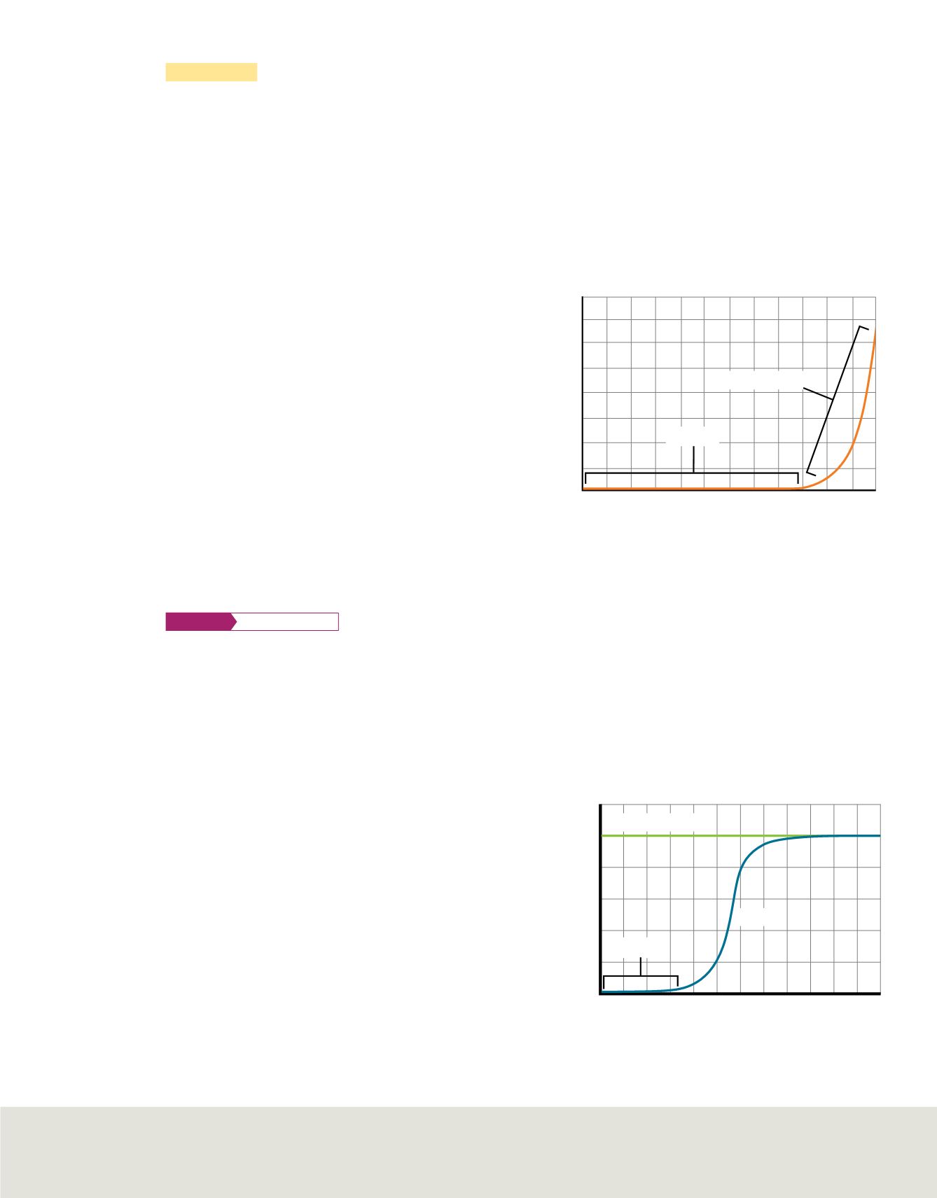
Logistic Population Growth
S-curve
Lag phase
Carrying capacity
2000
0
4000
6000
8000
10,000
Population
Time period
25 23 21
19 17 15 13 11 9 7 53 1
Immigration
(ih muh GRAY shun) is the term ecologists use to describe the number of
individuals moving into a population. In most instances, emigration is about equal to
immigration. Therefore, natality and mortality usually are the most important factors in
determining the population growth rate.
Some populations tend to remain approximately the same size from year to year. Other
populations vary in size depending on conditions within their habitats. To better
understand why populations grow in different ways, you should understand two mathe-
matical models for population growth—the exponential growth model and the logistic
growth model.
Exponential growth model
Look at
Figure 7
to see how a population of mice would grow if
there were no limits placed on it by the
environment.
Assume that two adult mice breed and produce a
litter of two young. Also assume the two off-
spring are able to reproduce in one month. If all
of the offspring survive to breed, the population
grows slowly at first. This slow growth period is
defined as the lag phase. The rate of population
growth soon begins to increase rapidly because
the total number of organisms that are able to
reproduce has increased. After only two years,
the experimental mouse population would reach
more than three million mice.
Notice in
Figure 7
that
once the mice begin to reproduce rapidly, the graph
becomes J-shaped. A J-shaped growth curve illus-
trates exponential growth. Exponential growth, also called geometric growth, occurs when
the growth rate is proportional to the size of the population. All populations grow exponen-
tially until some limiting factor slows the population’s growth. It is important to recognize
that even in the lag phase, the use of available resources is exponential. Because of this, the
resources soon become limited and population
growth slows.
Logistic growth model
Most populations
grow like the model shown in
Figure 8
rather
than the model shown in
Figure 7
. Notice that
the graphs look exactly the same through some
of the time period: the number of individuals
begins very low, then increases very rapidly.
During this period, competition for resources
among individuals in the population is low.
The second graph, however, curves into the
S-shape typical of logistic growth. Population
growth stops increasing when an environment's
carrying capacity has been reached.
Figure 7
If mice were allowed to reproduce unhindered,
the population would grow slowly at first but would
accelerate quickly.
Infer
why mice or other populations do not continue to
grow exponentially.
Figure 8
When a population exhibits growth that results in
an S-shaped graph, it exhibits logistic growth. The population
levels off at a limit called the carrying capacity.
MATH
Connection
Lesson 1 • Population Dynamics
83